Data
Kit results are shown in Data.
Select data

→ refer to section Load results
Context settings

After loading data, user-selected settings made in Results > Data can be saved as a "context setting".
- To loaded results apply user-selected settings, e.g. for "Data normalization" or "Metabolism indicators".
- To save these user-selected settings, click
.
- Define a name for this "context setting", in this example "Quant 500 XL export".
 Click Save.All user-selected settings are saved, e.g. as "Quant 500 XL export".
- If changes were defined compared to loaded context settings, the
symbol turns red →
.
- To save the current user-selected settings as new context settings, click on the
and define a new context setting name.
Options
Select
Reset
Delete
Example

Value type

The displayed values of results can be defined. The default value is: concentration in the unit µmol/L.
Results can be displayed using different reporting values, that can be chosen from a dropdown menu.
| Display value | Description |
|---|---|
| Concentration | Metabolite concentration in the specified unit (default μM) |
| Analyte intensity [cps] | Analyte signal intensity in counts per second (cps) |
| Internal std. intensity [cps] | Internal standard (ISTD) signal intensity in counts per second (cps) |
| Intensity ratio | Analyte signal intensity to ISTD signal intensity ratio |
| Accuracy [%] | Accuracy of measurement given as percentage: Measured concentration / expected concentration × 100 |
| CV [%] | CV given as percentage of quality control samples, run in replicates of three or more per plate run |
| Analyte peak area [area] | Integrated peak area of analyte |
| Internal std. peak area [area] | Integrated peak area of ISTD |
| Area ratio | Analyte peak area to ISTD peak area ratio |
| Analyte retention time [min] | Retention time of analyte based on chromatogram apex |
| Internal standard retention time [min] | Retention time of ISTD based on chromatogram apex |
| Relative retention time [min] | Ratio between analyte and ISTD retention time |
| Analyte peak width [min] | Peak width (full peak width) of analyte, given in minutes |
| Internal std. peak width [min] | Peak width (full peak width) of ISTD given in minutes |
| Analyte peak width at half height [min] | Full width at half maximum (FWHM) of metabolite peak. |
| Internal std. peak width at half height [min] | Full width at half maximum (FWHM) of ISTD peak. |
| Intensity-to-peak area ratio | Ratio between metabolite peak intensity (peak height) and peak area |
| Internal std. intensity-to-internal std. peak area ratio | Ratio between ISTD peak intensity (peak height) and peak area |
| Intensity-to-peak width ratio | Ratio between metabolite peak intensity (peak height) and peak width (full peak width) |
| Internal std. intensity-to-internal std. peak width ratio | Ratio between ISTD peak intensity (peak height) and peak width (full peak width) |
| Area-to-peak width ratio | Ratio between metabolite peak area and peak width (full peak width) |
| Internal std. area-to-internal std. peak width ratio | Ratio between ISTD peak area and peak width (full peak width) |
| Peak start height [cps] | Intensity at the starting point of peak integration |
| Peak end height [cps] | Intensity at the end point of peak integration |
| Peak symmetry | Degree of analyte peak symmetry. symmetric = 1 | not symmetric = < 1 or > 1 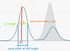 if a > b: between 1 and ∞ | if a < b: between 0 and 1 |
| Internal std. peak symmetry | Degree of ISTD peak symmetry. 1 when symmetric. |
| Peak resolution | Separation degree from next eluting peak. 1.5 when baseline separated. |
Display options

Define displayed options of loaded results, that can be chosen from a dropdown menu.
| Display value | Description |
|---|---|
| Sample types | Select a sample type, e.g. "Sample" |
| Show class | Display metabolites of the selected class |
| Show bio ID | Display bio IDs and links to bio ID databases, Note: Not all metabolites are available in every database. Some metabolites may have multiple entries |
| Show analytical details | Displays quantification limits (ULOQ, LLOQ) and further details. Show calibrator usage, included calibration standard levels Show calibration equation of calibration curve |
| Sort columns by | Class and name: Sort by metabolite class then name Name: Sort alphabetically by metabolite name |
| Concentration unit | Specify concentration unit of results. For tissue normalization: pmol/mg Tissue For cells normalization pmol/10E6 Cells |
| Log transform data | log2 or log10 log transformation |
| Split merged rows | Show results from different kit runs in separate rows |
Preprocessing

Preprocessing is a toolset that performs data cleaning and missing value imputation on results before exporting. This process helps to create a more robust dataset for downstream statistical analysis.
Data processing is optional. Imputation is exclusively applied to unknowns (study samples).
Preprocessing options
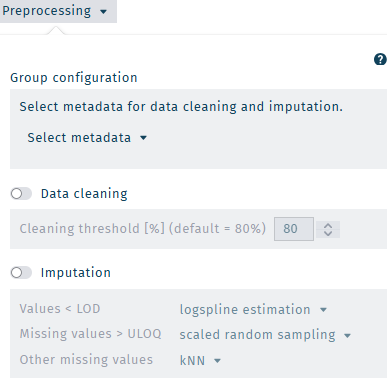
Group configuration
Data cleaning is performed based on the dataset's defined group information.
- Metadata is specific for the loaded results and is defined for "unknowns" during sample registration, see section groups and variables.
- If no metadata is selected, all loaded samples are treated as one group.
Example | Combined (concatenated) metadata
- Metadata from different categories can be combined.
- Samples with linked metadata categories "Gender" and "Treatment" is loaded, containing two groups each,Gender: "m" and "f"Treatment: "treated" and "control"
- If one of both categories "Gender" or "Treatment" is loaded, for data cleaning two groups are used:"m" and "f" or "treated" and "control".
- If both categories "Gender" and "Treatment" are loaded, for data cleaning a combination of categories and groups is used: "m-treated", "f-treated", "m-control", und "f-control"
Data cleaning
To improve the reliability of any statistical findings during the later evaluation, the function of data cleaning is to remove metabolites that are not well detected across all groups in the study.
- A cleaning threshold is defined to remove metabolites from the loaded dataset that are not suitable for further processing.
- A cleaning threshold of 80% will remove metabolites from a dataset ifless than 80% of concentration values for one metabolite are valid andthis applies to all groups.ExampleA) Valid concentrations in 75% of samples in group A, 79% in group B → the metabolite is excludedB) Valid concentrations in 80% of samples in group A, 0% in group B → the metabolite is not excluded
- Concentrations are evaluated metabolite by metabolite, based on the group configuration.
Applying the "80/20 rule"
- The "80/20 rule" uses a cleaning threshold of 80%.
- Concentrations are evaluated based on the group configuration for each defined metadata individually, e.g., for the combination of the metadata information "Material" and "Species".
- The evaluation is performed metabolite by metabolite to each metadata set. The "80/20 rule" is applied: if more than 20% of concentrations in all groups have non-valid concentrations, e.g. < LOD, the metabolite is excluded from the loaded results.
- Removed metabolites are not displayed in Results > Data. (For removed metabolites, no specific status is given as they are are absent from results.)
- Imputation is only applied to metabolites that were not removed.
Imputation
Imputation is a process that replaces unusable or removed values (defined below) before any further data processing is performed, such as statistical analysis.
Definitions
Imputation can be performed for the following categories of unusable values.
Values < LOD/2 are imputed with values between LOD and LOD/2 using a logspline probability function, preserving the variance within the dataset and taking the distribution of values between LOD and LOD/2 into account.
Missing values > ULOQ, e.g. "∞", are replaced by a random number higher than the largest usable metabolite specific concentration value of the dataset but lower than its double within the interval between the max value and 2-times the max value.
Other missing values are missing at random for technical reasons. They are imputed with the k-nearest neighbors (knn) algorithm.
Normalization

For the long-term comparability of results, normalization is a crucial procedure. Normalization has been shown to reduce cross-batch variability, improve inter-laboratory reproducibility, and increase data accuracy. The recommended procedure is target value normalization using QC 2 as sample source, which is applied by default.
ⓘ For technical details of the normalization procedures, refer to the Appendix > Normalization.
It is strongly recommended to normalize all results!
Recommended normalization procedure: target value normalization and QC 2 as sample source
Replicates for normalization
The effectiveness of normalization procedures was demonstrated during inter-laboratory ring trial studies.
biocrates kit ring trial publications
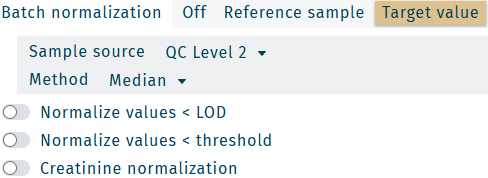
Available Normalization options applied to loaded results.
| Display value | Description |
|---|---|
| Batch normalization | Define the normalization algorithm and sample source → Batch normalization |
| Normalize values < LOD | Normalization is performed for concentrations with the status "< LOD". |
| Creatinine normalization | For urine samples: metabolite concentrations are divided by creatinine concentration of the respective sample. |
| Subtract median concentration of zero samples | For e.g. supernatant from cell culture: The median concentration of zero samples is subtracted from the metabolite concentration of unknowns. ⓘ To subtract metabolite concentrations of cell culture medium from unknowns, use “unprocessed” medium as zero sample. This may also be used for samples with very low metabolite concentrations, like cerebrospinal fluid (CSF). |
Batch normalization
- Off
- Reference sample
- Target value
No normalization is performed.
Inter plate run (kit run) normalization is performed, based on average concentrations of the selected reference sample.
Requirements
Intra plate run (kit run) normalization is performed, based on average quality control (QC) metabolite concentrations of the selected QC.
Requirements
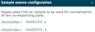
Sample source
Configuration
Method
Matrix specific normalization
Perform a sample material or species specific normalization when material or species specific QCs where measured.
If more than one Custom QC was loaded together with study samples (unknowns), to define a specific Custom QC for the normalization procedure use the option configuration.

Example
ⓘ Normalize each sample matrix separately, e.g. 1. plasma and 2. tissue samples.
1. Normalization of plasma samples
- Exclusively load plasma study samples ("unknowns", material = plasma) and biocrates QC (material = plasma), according to section Load results > Sample selection options, select samples, material = plasma.

- Define normalization, according to section Data normalization. Define optional options like preprocessing, if desired.
- Export results.
2. Normalization of tissue samples
- Exclusively load tissue study samples ("unknowns", material = tissue) and Custom QC (material = tissue), according to section Load results > Sample selection options, select samples, material = tissue.
- Define normalization, according to section Data normalization. Define optional options like preprocessing, if desired.
- Export results.
MetaboINDICATOR

MetaboINDICATOR is a tool that calculates sums and ratios of metabolites with relevance to biological and clinical applications (metabolism indicators), to support a more comprehensive understanding of metabolomics studies. In addition, these indicators can significantly reduce biological and analytical variability and can improve the specificity of many findings.
The MetaboINDICATOR tool provides a set of pre-configured sums and ratios that proved to be particularly informative on certain clinical conditions or pathophysiological events. In addition, user-defined sums and ratios can also be created. All sums and ratios are automatically calculated and displayed at the end of the Results table.
A list of all metabolism indicators can be found in the product-specific document biocrates-kit list of metabolite sums and ratios (v#-yyyy).xlsx on the Kit files.
If sample data was loaded, but metabolism indicators are not available
Example for Quant 500 XL kit, SCIEX 5500+
Select metabolism indicators
Categories for specific diseases, lifestyle factors, and physiological functions

Two display options for metabolism indicators are available, as table or grouped.
| Table | Grouped |
|---|---|
 |
- To display or hide metabolism indicators, use the toggle
.
- To search for specific categories, the filter may be used.
Change view option "table" or "grouped"
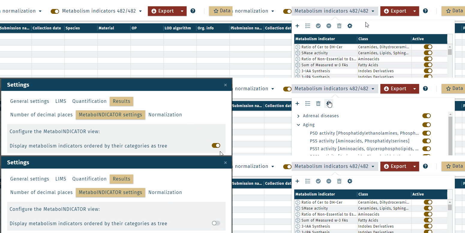
Display or hide metabolism indicators
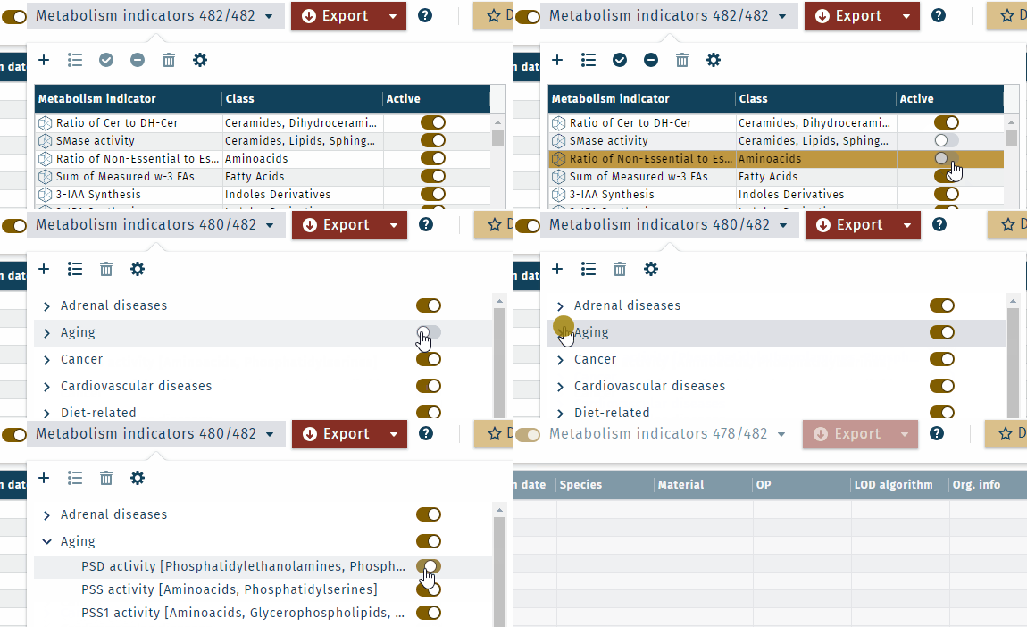
In table view, multiple indicators or a category can be activated or deactivated simultaneously.
- To select specific metabolism indicators, use "shift-click" to select a range or"control-click" for individual selections.
- To activate or deactivate all selected, use the
or
buttons.
All metabolism indicators can be displayed collapsed or expanded.

Metabolism indicator number
- The number of available metabolism indicators depends on the loaded dataset and is the second number shown, e.g. 281.
- Metabolism indicators can be activated or deactivated, → Display or hide metabolism indicators.
- The number of activated metabolism indicators is the first number shown, e.g. 280.
The number of available metabolism indicators (the second number shown) depends on the loaded dataset. It may be lower than the maximum number.
Metabolism indicator status
- Metabolism indicators receive a status based on the corresponding single concentration statuses, like "valid" or "< LOD", see concentration validation status, list item 4.
- The status of hightest priority is used for a metabolism indicator (MI). Example: MI = A + B + C. Status of A and B are "valid" and of C is "< LOD". The status of MI is "< LOD".
- Sums are calculated if at least one of all summands or subtrahends is different from a zero value. Otherwise the sum is removed.
- If one summand or subtrahend is missing, the metabolism indicator status is "Incomplete metabolism indicator" and calculated.
- If the enumerator or denominator of a ratio is zero (no concentration available), the ratio is removed (not displayed).
- If imputation was performed, imputed concentrations are included in metabolism indicator calculations.
ⓘ The metabolism indicator status is independent from imputed or non-imputed concentrations.
Metabolism indicator details
- To see additional information, such as formula, description, and literature references, select a metabolism indicator and click the info button
.
- Metabolism indicators pre-defined by biocrates are highlighted with the biocrates logo
.
- Metabolism indicator "categories" or "analyte classes" can be shown in the results table, which is defined in the Settings.
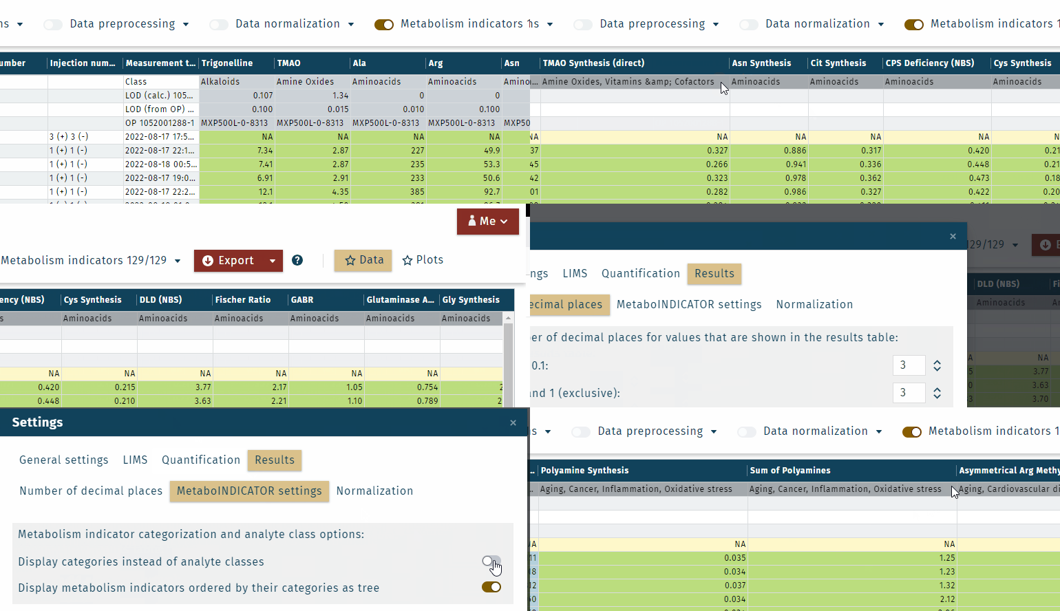
Custom metabolism indicators
MetaboINDICATOR also supports user created custom metabolism indicators.
To create a new indicator, click the icon in the MetaboINDICATORs dropdown menu.
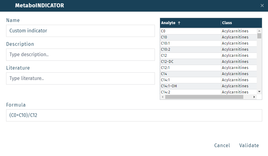
In the MetaboINDICATOR window, give the custom indicator a name (i.e. "Custom indicator"). Enter the formula for the indicator in the Formula field (i.e. (C0+C10)/C12). The list of possible metabolite names can be seen in the table on the right side. The formula can be constructed using standard arithmetic operators: +, -, *, / with parentheses to define the order of operation.
Once the formula has been entered, click Validate to check the validity of the formula. If the formula is OK, click Add to save the indicator.
To edit a custom indicator, select and click the info button . To remove, use click the trash icon
.
Metabolism indicators pre-defined by biocrates are highlighted with the biocrates logo .
Export

To export results click Export.
→ for details refer to section Export results